|
Stephanie's Homepage
|
Unblinding Discussion
Unblinding proposal slides.
Diffuse call
- Referee 1: Lisa Gerhardt
- Referee 2: Dima Chirkin
Thursday 3rd February 2011, 7:00am
Lisa: In all level 4 plots the data seems to be above the CORSIKA, but Table 1 at the bottom of the page shows the CORSIKA rate as being higher than the data. Is this correct?
It actually is correct, although I have made it look a little confusing. The rate in the table is referring to AFTER level 4 cuts. At this cut level Monte Carlo rises above data due to the cuts being in a region that allows this to happen. The plots you see on this page are showing where the level 4 cuts are placed, so are from BEFORE the actual cuts are made. To see plots that show the data/Monte Carlo discrepancy at this level refer to my Level 5 webpage.
Dima: Why is the reconstructed vertex position situated towards the edges of the detector for background? e.g. Credo_Vertex_Z in TMVA input variables.
At this level the remaining background events are muons that have passed the previous cut levels. In order for these muon events to have survived they must have "cascade-like" properties such as slow linefit velocity, spherical topology, large fill ratio, etc. Muon events that have these "cascade-like" properties are more likely to be events that are close to the edge of the detector. One way to remove these events would be a containment cut, however a dedicated containment cut sacrifices too much signal in a high energy analysis for IC40. These events are removed using alternative cuts and contaiment like cuts before and inside TMVA.
Spencer: Can you make the TMVA plots for each variable showing the data and Monte Carlo to compare the distributions? (rather than just signal and Monte Carlo)
Yes, I have done this by substituting the 10% burn sample data into TMVA in place of the signal. This makes no sense in terms of analysis of course, but does show the differences between the data and CORSIKA in each variable and overall very well. You can find all the plots from the TMVA output in the second section of my Data/Monte Carlo Comparison webpage.
Spencer: Can you show the expected signal from atmospheric neutrinos? This may make a big difference to your final sensitivity.
Yes, I have added in the atmospheric neutrino signal into all plots. The final rate for this signal is 1.19896 × 10⁻⁷Hz which gives an expectation of 3.49 events. I have added into my calculation for sensitivity.
Spencer: Since you have run out of double CORSIKA by the final level of the analysis, are you able to estimate the double CORSIKA upper limit?
I have specific cuts at earlier levels in my analysis (especially levels 4 and 5) that are very effective at removing coincident events so I think I have sucesfully eliminated double CORSIKA rather than just running out of statistics. However, I can estimate an upper limit by using the ratio of the DiplopiaWeight for single and double CORSIKA, e.g. (Ratesingle / DiplopiaWeightsingle) × DiplopiaWeightdouble = Ratedouble which can be used to estimate the number of double CORSIKA events in the usual way, which I have also done for triple CORSIKA. You can find these numbers on my Final webpage. However, since this question was asked I have added more stringent containment cuts which has reduced my background due to muons to zero at final level.
Kurt: Can you double check that your remaining data event 110860 is not a flasher event?
All my runs are "good" runs according to the IC40 good run list so there should be no flasher events included. To confirm this I have checked run 110860 on IceCube Live to make sure that there is no record of Light In Decector (LID). In addition, I have checked that all DOMs around the vertex are read out. This is a robust way to check the event is not a flasher since in flasher events the flashing DOM is absent from the IC40 geometry. The reconstructed vertex of this event falls somewhere around DOM 18 and between strings 63, 70 and 71. The following DOMs were read out from InIceRawData:
String 63: DOMs 9, 11, 12, 13, 14, 15, 16, 17, 18, 19, 20, 21, 22, 23 ,24, 25, 26, 27
String 70: DOMs 10, 11, 12, 13, 14, 15, 16, 17, 18, 19, 20, 21, 22, 23, 24, 25, 26
String 71: DOMs 12, 13, 14, 15, 16, 17, 18, 19, 20, 21, 22, 23, 24
String 62: DOMs 12, 13, 15, 16, 17, 18, 19, 20, 21, 22, 23, 24
String 64: DOMs 14, 15, 16, 17, 18, 20, 21, 22, 23, 24
String 55: DOMs 15, 16, 18, 19, 21, 22, 23, 24
String 76: DOMs 17, 18, 21, 22
String 54: DOMs 22, 23
String 69: DOMs 13, 14
Lisa: Can you use a dataset for tau neutrino signal simulation that is not UHE?
Yes. I was using the wrong dataset as this one was initially the only tau neutrino dataset available for this analysis. There is now another dataset that is not UHE which has different cross-sections (dataset 5117). I am now using this one, and have updated all my plots and calculations accordingly.
Kurt: Are there datasets with the new cross-sections for IC40, and are you able to use these for a systematic study?
There are some datasets with the new cross-sections for IC40 and I am planing on using them for systematics. You will find the results of this systematic study (when complete) on my Systematics webpage.
Spencer: Can you make plots for each of the TMVA variables? This will show if any variable in particular is contributing to the shape discrepancy between data and CORSIKA.
Yes, I have done this. You will find these plots in Figure 2 on my Level 5 webpage. All variables show CORSIKA as having a higher overall rate compared to data as expected, however none of them stand out as having a large discrepancy in shape.
Kurt: Can you optimise your final level using sensitivity (MRF and MDF) rather than S/&radic(S+B)?
Yes, I have now done it this way. I use &nue signal and CORSIKA to do this optimisations, you will find all the details on my Level 6 webpage.
Kurt: Can you put a link somewhere to the plot comparing the energy range of each IC40 analysis that you made earlier?
Yes, you will find a link on my main analysis page to this comparison of IC40 analyses energy ranges plot.
Email from Joanna, Saturday 12th February 2011, 8:35pm
I'm puzzled that after your level4 cut the corsika rate seems higher that the data (could you please add statistical uncertainties on the rates?) I don't think we've seen it before ... Wouldn't a simple cut on Zenith (before training) http://www2.phys.canterbury.ac.nz/~svh13/level5/tmva-variables/IC40_L4_Cascade_1d_Zenith_Plot.gif make data and corsika agree better (both in absolute rates and shapes)? I suggest it, because at teh later stages of your analysis: http://www2.phys.canterbury.ac.nz/~svh13/level5/IC40_L4_Cascade_1d_BDTresponse_Plot.gif one cannot really justify making a cut on a variable whose distribution is different for the data and MC ... If modifying cuts at earlier levels (level4) doesn't help, splitting the data by depth, reconstructed energy, nchannels, fill-ratio , etc may help to understand where this discrepancy may come from. Perhaps you can apply certain cuts (e.g. some or all cuts from your level6) earlier in your analysis?
The CORSIKA rate ends up higher than the data after my level 4 cuts because of the region of parameter space that I am cutting in. You can see this in the plots on my level 4 page. I throw out regions that have a data much higher than CORSIKA and keep regions where the CORSIKA is higher than the data. I have now changed my TMVA to include three precuts:
CredoFit4_Pos_Z > -450 metres and < 450 metres
String containment
DOM charge containment
This improves the agreement in shape between data and CORSIKA for the BDT response variable, although there is still some discrepancy. You will find all my updated plots on the usual Level 5 webpage.
My remaining comments below are for http://www2.phys.canterbury.ac.nz/~svh13/final.html: The tau effective area looks strange to me. Why there are no entries below log10(E/GeV)~9?
This is because the tau neutrino dataset that I am using is a UHE one so only turns on at log10(E)=9. This is the only one available with the cross-sections that I use. However, there is a tau neutrino dataset that has normal energy range with the newer cross-sections. I was asked about this in the diffuse call have switched to this new dataset.
How do you count signal events in http://www2.phys.canterbury.ac.nz/~svh13/final/IC40_Final_Cascade_IC22_Comparison_Plot.gif? Is the number of signal events for your analysis shown in this figure consistent with numbers in Table I? I'm confused by the ic22 numbers (for the lifetime of 257 days tehre are 14 events left - I don't see it from your plot) Why the last two bins are shown as horizonal lines?
The numbers for my IC40 analysis in this plot are similar to those in the table but have an assumed flux of (1 × 10⁻⁶ GeV sr-1 s-1 cm-2, the same as your IC22 analysis. I did take the numbers for your IC22 analysis from your webpage, but have now changed to the values from your paper (these are almost the same anyway). The last two entries were horizontal lines rather than points because you have no data events left at these levels. These levels don't really fit on this plot in that sense, but I put the lines there to give an indication of where the signal events lie. I have now removed these two entries since they are not present in your paper.
Why do you use as a reference flux 4.1 x 10^-7 (Oxana's "old" - i.e. not the one that is published - limit)?
I didn't realise this was the old one and not the published limit. I assumed it was correct since it is what Sebastian is using. I have since learned that the IC22 limit is in fact better (3.6 × 10⁻⁷ GeV sr-1 s-1 cm-2) so I have changed my final numbers accordingly.
Please remove (10%) from Table I.
Done. I had this as an indication that the number of events is estimated from 10% of the data, but I agree that it made it look confusing.
Could you please add reconstructed cascade energies for corsika events?
The reconstructed energies are already there (from CredoFit4) - it is the first energy that I quote. The second two energies are the MCtrue ones, they are the ones in the brackets. However, since answering this question I have added more stringent containment cuts which has reduced the CORSIKA background to zero at final level.
Thursday 17th February 2011, 7:00am
Lisa: Can you check if any of your remainig data events have an IceTop trigger?
Yes, I have checked this. There are no pulses from IceTop for any of my remaining data events.
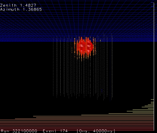
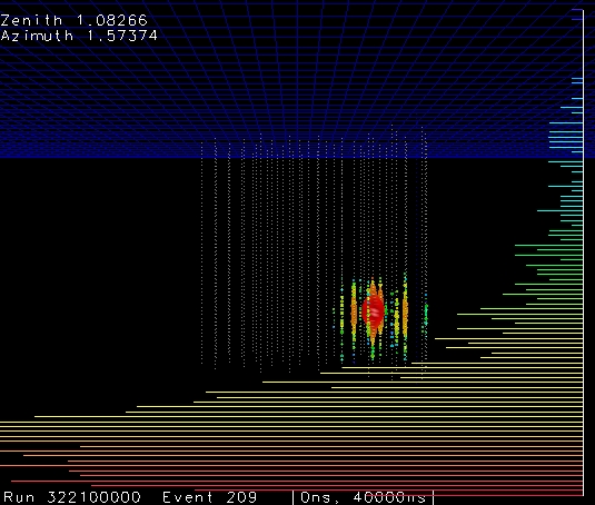
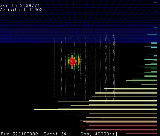
Kurt and Lisa: Can you look at the remaining simulated signal events to see where they lie in the detector (x, y and z vertex position) and to see if your remaining data events look like the simulated signal?
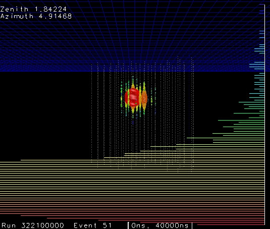
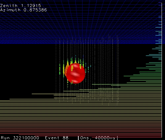
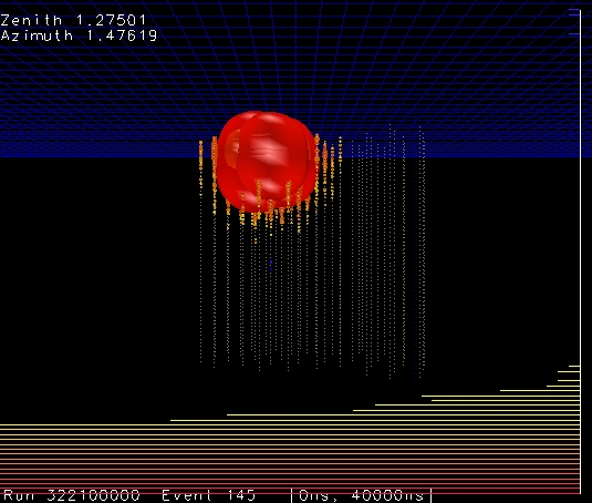
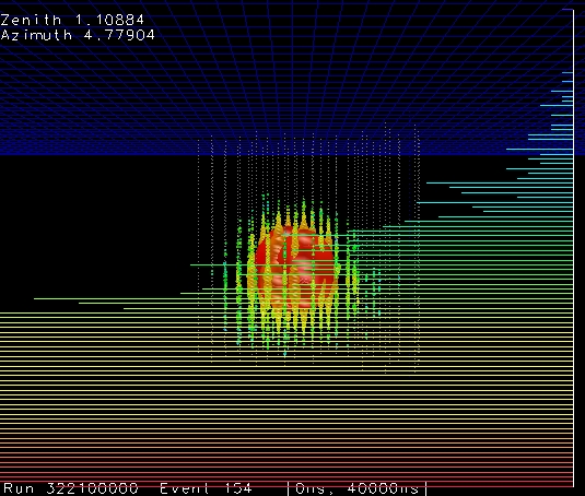
Below you will see three 1d plots showing the reconstructed x, y and z vertex positions, and a 2d plot showing the x-y arial view of the detector (for data and CORSIKA as well as the requested signal). The reconstructed vertex position for signal is flat in all x, y and z distributions, with no particular preferred locations. I have also shown some event viewer displays of "typical" (there are 110,575 simulated signal events left) signal events.
 |
 |
 |
 |
 |
 |
 |
 |
 |
 |
 |
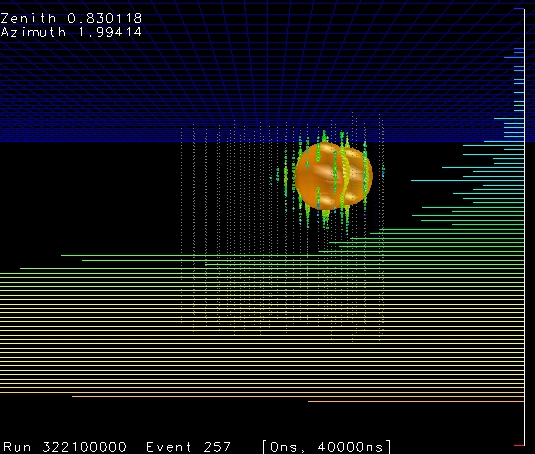 |
Figure 1: After final level of cuts using CredoFit4: a) Reconstructed x vertex position, b) Reconstructed y vertex position, c) Reconstructed z vertex position, d) Reconstructed x-y vertex position view from above, e), f), g), h), i), j), k) and l) Event viewer displays of "typical" simulated signal events.
Patrick: Every remaing CORSIKA event has its largest energy deposited on an outside string. Why do you not have a containment cut? This would get rid of all of your background without rejecting either of your remaining data events.
Due to the IC40 geometry background muon events that survive to the final stages of the analysis (corner clippers) are more likely to reconstruct at the edges, in particular at the top and bottom of the detector and at the "pointy" corner (string 21). It is for this reason that I do have containment cuts on these areas. I restrict CredoFit4_Pos_Z and CredoFit4_Pos_X and CredoFit4_Pos_Y in my precuts to TMVA, as well as now a more stringent containment cut on the position of the DOM with the largest charge.
I looked extensively into doing a x-y containment cut at earlier cut levels. For a high energy analysis with IC40 geometry this type of cut has very bad signal efficiency compared to other cut variables. In addition to my precuts for TMVA I also a cut variable that goes into the TMVA training which is equivalent to a containment cut. I call this variable Split Containment on my Level 5 webpage. It gives the distance of the reconstructed vertex position from the centre of the detector using only the first half of the hits. You can see from the plot that background does indeed reconstruct closer to the edge of the detector than signal, and that this variable has high discriminating power for TMVA.
Thursday 17th March 2011, 6:00am
Lisa: Will Sebastian's events pass your analysis?
No, they will not. 3 out of 4 of his events do not pass my reconstructed z vertex cut because they are either too high or too low in the detector. This is a precut to TMVA so these events do not even make it into my training. In addition to this if one is worried about events similar to this passing my analysis (such as events that just pass my containment cuts) I do not think these would pass either. This is because I run 4 iteration Credo in my processing instead of only 1 iteration. This means my energy estimation is better, and so it is less likely that I will have the problem of corner clippers passing my analysis cuts due to their energy being reconstructed unrealistically high.
Lisa: Can you make the resolution plots for CORSIKA (at lower levels) for only events that are outside the detector? This is to check the performance of 4 iteration Credo compared to 1 iteration Credo for these types of events.
I can not make the resolution plots for CORSIKA since there is no true cascade quantaties. I can however use the signal events that are outside the detector. You will see these plots in Figure 2, I have used cuts on vertex position at x < -400 metres, x > 450 metres and y > 450 metres. There is no cut on the lower bound of y vertex position or on z vertex position since these events are cut away by my precuts to TMVA. These plots show clearly that 4 iteration Credo does indeed perform substantially better than 1 iteration for events outside the detector as well as inside. These events are of course not in my final event selection since I have containment cuts.
 |
 |
 |
 |
 |
 |
Figure 2: Uncontained resolution plots a) X vertex, b) Y vertex, c) Z vertex, d) Energy, e) Zenith, f) Azimuth.
Lisa: What would a containment cut do to this analysis?
Patrick asked this same question at the 17th February diffuse call. See the answer above.
Allan: Can we get Patrick to look at the remaining data events with his python event viewer in the same way that he did with Henrik and Sebastian's events?
Yes, I have emailed him about this and he has kindly looked into my remaining events. I have added his python event displays to my Final webpage.
Spencer: Why is your discovery flux greater than your sensitivity flux?
Sorry, this was a typo. It is suppossed to be 10-8 not 10-9, I have corrected this in the table.
Gary: Can you make n-1 plots of all cut variables after final level? This is to see where the remaining data events lie in these distributions. i.e. Do they lie very close to the cut boundaries, or are the parameters of these events really inside the cut boundaries meaning we can be more confident that they are actually cascade events?
Yes, I have done this for level 6 variables. You can find these plots added to my Final webpage.
Spencer: You need an estimation for double and triple CORSIKA that is not 0 events. Can you increase the number of decimal places that you quote these values as in your table?
They are only 0 events to a precision of two decimal places. I have increased this to four decimal places so you can see that the estimate for double and triple CORSIKA background is not really 0 events. However, since doing this I have applied more stringent containment cuts, which has in fact reduced my CORSIKA background to zero events at my final level. There is still an uncertainty on this value of zero found by systematics studies.
Spencer: Can you add in atmospheric background from muon neutrinos as well as electron? The contribution from this background may be significant.
Yes, I have done this. Atmospheric muons do make a significant contribution to the background, and I have updated my sensitivity calculation on my Final webpage accordingly.
Gary: What about doing a likelihood fit on the final spectrum?
You have asked this question before to other analysers. :) To use this method in an analysis one really needs to decide to do it from an earlier stage, so I think it is too late to change to this method for my analysis now. I am also of course under some time constraints to unblind and finish my PhD.
Spencer: Can you make a plot showing the effective livetime of your CORSIKA as a function of energy?
Yes, I have made several plots of the effective livetime for my CORSIKA. You will find these added to my Final webpage.
Kurt: What is the fudge factor for your analysis at the highest cut level?
At the final level, the definition of the fudge factor (RateData/RateMC) is ambiguous, since most (or all) events in the data are signal, not background. The rate of background events in the data is then really 0Hz so the fudge factor is undefined. I actually do not apply any fudge factors to any of the plots that you see, however I do track the data/MC normalisation throughout each level of my analysis, and you can see this on my Data/Monte Carlo Comparison webpage. The data/MC is ~1.5 at levels 2 and 3, it then drops to ~0.8 at level 4 and 5 (low statistics already so data contains substantial signal events). The data/MC is used in determining the systematic errors for this analysis, you will find the details on my Systematics webpage (when complete).
Email from Henrik, Thursday 17th March 2011, 7:18am
Do you plan on using neutrino simulation with the new CSS cross sections for all flavors?
No, I don't. I was initially only using neutrino simulation with hteq, however I switched to CSS for tau neutrino as hteq was never produced. Electron and muon neutrino datasets using CSS cross-sections have not been processed to level 3 for the cascade stream. The one exception is a small electron neutrino dataset (5102 which is only 500 files) which intend to use for a systematics study into cross-sections for this analysis.
Have you looked at the predicted number of events from atmospheric muon neutrinos? There might be a significant contribution from neutral current events.
Yes, I was also asked about this in the diffuse call this morning. Atmospheric muons are a significant contribution to the background, and I have now updated my final calculations for sensitivity with this included.
It looks like the MRF is calculated using the total signal prediction from all neutrino flavors. And it looks like the normalization of the signal flux is 3.6e-7 for each flavor. The all-flavor signal flux normalization would then become 3*3.6e-7. So for the sensitivity one would then get MRF*3*3.6e-7, which is 3 times higher than the sensitivity shown in table 2.
Yes, you are correct. I had missed this factor of 3 from my calculation. I have now corrected this and updated the values.
Email from Lisa, Thursday 17th March 2011, 10:05am
I was looking at the event views of "typical" simulated events on this page http://www2.phys.canterbury.ac.nz/~svh13/unblindingDiscussion.html and it seems like all of these events have really huge energy deposits in the center of the cascade. Did you think about some kind of cut that looks at the ratio of maximum charge over total charge? Probably you already have, but I wanted to mention it just in case.
I did look into this earlier on in my analysis but decided against it. Not all the signal events look like this - those I show above are the first 8 out of 110,575 events left at my final level. There are many other events that do not have this topology or that have multiple DOMs with very large energy deposits. Also, there are muon background events that show this behaviour. This variable is also not stored in my flatnt rootfiles so to go back and re-look at it I would have to reprocess from level 4 onwards which is not realistic at this stage.
Also, I was looking at this plot of the BDT: http://www2.phys.canterbury.ac.nz/~svh13/level5/IC40_L4_Cascade_1d_BDTresponse_Plot.gif There's a large shift between the data and the total corsika estimates. If you took the total corsika distribution and shifted it to the right until it agrees with the data, how much does the expected number of events from corsika increase?
It is not really justified to shift this plot, since the BDT response is not a physical quantity. The discrepancy between data and CORSIKA improves with cleaner event samples, below is a plot showing the BDT response with an additional cut on Energy. This plot shows that the discrepancy between data and CORSIKA has improved (a lot) and the shift has dissapeared with this addional cut so one can trust the BDT response variable in the parameter space that my analysis is in. It is not possible to apply the all the final cuts before the TMVA training since the algorithm requires higher statistics to train on.
 |
Figure 3: BDT response after final level cuts.
Phone call with Kurt and Gary, Friday 18th March 2011, 7:30am
Can you make the 2d plot of x vertex position vs. y vertex position after level 5? This is so we can see where events lie with higher statistics before the final cut level.
Yes, this plot is shown below. The IC40 string positions are shown by the black dots. The majority of both data and CORSIKA events are contained within the detector. There is maybe some evidence that the events are clustered towards some of the edges or sharp parts of the detector. Since making this plot I have added in more stringent containment cuts so this is now obsolete (see question below).
 |
Figure 4: Reconstructed vertex position.
Although a containment cut does not work at lower levels, can you look into this at the final level to reduce the CORSIKA to 0 events with certainty?
Yes, I have worked on this. I now have two types of containment cuts which are precuts to my TMVA training at level 5. The first is on the reconstructed vertex position, which I require to be inside the detector volume. The second is on the position of the DOM with the largest charge, which I require to be not on an outer string. This second containment cut is really just a more stringent version of the first. These two cuts do indeed reduce my final CORSIKA background to zero by final level.
Email from Henrik, Thursday 19th March 2011, 12:33am
I understand that you are very busy, I just wanted to mention one more thing I noticed. I wanted to make sure I wasn't jumping to conclusions so I had a closer look at your effective area plot
http://www2.phys.canterbury.ac.nz/~svh13/final/IC40_Final_Cascade_Effective_Area_Plot.gif. I read off the actual values for the muon neutrino effective area (using a nifty program that reads off curves from plots). With these values I calculated the number of events an E-2 flux normalized to 3.6e-7 would give for a livetime of 8093.71 hours. I got 28 events, which is half of the number listed for E-2 muon neutrinos in table 1 on the final level page. I verified the calculation on Sebastian's and my own effective area. So there might be a factor 2 missing somewhere, either in the expected number of events in table 1 or in the effective area plot.
Sorry for the late reply and thank you very much for pointing this out. The error is in my script that plots the effective area and I knew exactly what it was when you pointed this out. I have this line in my script:
TCut elecInverseNGeneratedFiles = "1.0/(2*5999)"; //2*Number of files (2 is average of nu and nuBar, otherwise will be the sum of the areas)
I was never really sure about that factor of 2. I asked a few people but no one really cleared it up for me. Thanks to you I now know what it should be. I have fixed this and updated my plot.
Email from Kurt, Tuesday 29th March 2011, 12:59pm
You quote an expected CORSIKA background of 0.03 events in 337 days of IC40. In comparison, Joanna's muon background was 5.4 events (after multiplication by the fudge factor 3) in 257 days of IC22. Given that her detector is half the size of yours, and she was using containment cuts (which you are not, yet), it seems strange that you expect two orders of magnitude less muon background.
Joanna actually has no CORSIKA events at her highest levels (7 and 8), I assume the value of 5.4 is including atmospherics. My total background is about 6 events when including atmospherics. Also, my analysis is very different to Joanna's. We have different cuts, in particular her energy was lower than mine.
The numbers from her paper draft are: 5.4 muons (estimated from four MC events) and 2.9 atmospheric neutrinos, at final level. This was after producing lots of additional high-energy-biased CORSIKA. Your numbers are: 0.03 muons and 5.9 atmospheric neutrinos. So getting about twice the number of neutrinos makes sense since the detector is about twice as large. But can differences in analysis and energy coverage really explain the factor 100 in muon background? Especially since your two CORSIKA events are on the edge and would not have survived her containment cuts (she required the four earliest hits to be inside the fiducial volume).
The energy cut can explain the difference between the background estimates. It makes more difference than one thinks. Below is a plot I made to try and illustrate this. The plot shows the number of surviving background (muon) events as a function of energy cut. You will see that if my energy cut were as low as Joanna's (4.2 logscale) I would have a comparable background to hers (~3 events). Since my optimum energy cut is 4.425 on logscale I have less than 1 event surviving. (Since answering this question my analysis has changed considerably due to adding a more stringent containment cut).
 |
Figure 5: Number of surviving background events.
If you expect 0.03 in about one year, then wouldn't the two CORSIKA events you are basing this estimate on correspond to hundreds (thousands?) of years of livetime?
Yes, this corresponds to a large livetime. I have made several plots showing my effective livetime and you will find these on my Final webpage.
Assuming that the background estimate is correct, can you calculate the signal flux that the five burn sample events would correspond to? It would be interesting to see if this is consistent with Joanna's limit.
This is already shown on my Final webpage. I calculate the signal flux and number of events using Joanna's limit. With her limit I would expect to see 66 events for the whole IC40 lifetime, which would be roughly 6 events in my burn sample. I have 3 events so this is well within her limit.
Thursday 31st March 2011, 6:00am
Allan: What would happen if you had a tighter containment cut?
This is an idea that has been proposed by a few people. I have added an additional containment cut to my precuts to TMVA at level 5. This cut is on the position of the DOM that has the largest charge in the event, which is required to not be on an outside string. This reduces my background to zero at final level.
Kurt: Can you change the tittle of Figure 3 on this page to be clearer?
Yes, this is done.
Lisa: What would happen if you had another containment cut later on?
This is an idea that has been proposed by a few people. I have added an additional containment cut to my precuts to TMVA at level 5. This cut is on the position of the DOM that has the largest charge in the
event, which is required to not be on an outside string. This reduces my background to zero at final level.
Henrike: Can you use the two-component CORSIKA that Henrik used in his analysis?
Yes, I can. These datasets are now included.
Email from Seon-Hee, Thursday 31st March 2011, 8:00am
I think only first two events among your final 4 events in the sample needs to survive by looking at them with the event-viewer. The last event does not look like cascade-like event. Thus I think it needs to be removed by applying a cut like TOI_evalRatio, for example. The 3rd event also does not satisfy containment condition in my eye. You'd better apply a containment condition that the string with maximum charge DOM is outer-most string then the event needs to be removed. I strongly recommend you to use this containment condition (based on my IC22 analysis experience).
Yes, I agree. I have now added an additional containment cut to my precuts to TMVA at level 5. This cut is on the position of the DOM that has the largest charge in the event, which is required to not be on an outside string. This reduces my background to zero at final level, and removes those events in the burn sample that look like they could be background sneaking through.
Phone call with Kurt and Gary, Sunday 3rd April 2011, 1:30pm
Can you make plots of BDT response with various energy cuts, and plots of energy with various BDT response cut?
Yes, the plots are shown below. The agreement between CORSIKA and data gets better in the BDT distribution with harder energy cut as expected. As the cut on BDT gets harder, the discrepancy between CORSIKA and data is always concentrated at the low energy end of the energy distribution. This demonstrates that the Data/Monte Carlo disagreements are confined to lower energies, as is seen by previous IceCube analyses so far. The agreement of data and CORSIKA gets much better with even a moderate cut of log10(CredoFit4_Eenegy) > 3.6.
 |
 |
|
 |
 |
 |
 |
 |
 |
 |
Figure 6: BDT response as a function of energy cut a) No energy cut, b) log10(CredoFit4_Energy) > 3.6, c) log10(CredoFit4_Energy) > 3.8, d) log10(CredoFit4_Energy) > 4.0, e) log10(CredoFit4_Energy) > 4.2. Figure 7: Reconstructed Energy as a function of BDT response cut a) No BDT cut, b) MVA_BDT > -0.10, c) MVA_BDT > 0.00, d) MVA_BDT > 0.10, e) MVA_BDT > 0.20.
Thursday 7th April 2011, 5:00am
Lisa: How do you do the optimisation for the final level?
I use Feldman-Cousins to calculate the MRF and MDF for cuts on BDT response and Energy. I use data to do this optimisation, since CORSIKA is lacking at high cut values. This has to be done carefully since the data may also contain signal events at high cut levels. You will see the output from this in Figures 3 and 4 on my Level 6 webpage.
Gary and Lisa: Can you make the BDT plot with a various energy cuts so we can see if this cut improves the data/CORSIKA agreement?
Yes, this was also asked on a phone call with Gary and Kurt. I have made these plots - you can see them in the above question (Figure 6).
Dima: Didn't you have a background of only 0.03 events last week - how come it rose to 4 events as in Table 2 on your Final webpage?
I did have 0.03 events from CORSIKA background last week - that has now dropped to 0 events. The 4 background events refers to atmospheric induced cascades.
Eike: Could you calculate the 90% mc_energy interval where your remaining nue events are?
The central 90% primary energy region is 4.4 to 6.7 in logscale. This is 25.12 TeV to 5011.87 TeV. I have added this information onto my Final webpage.
Kurt: Can you make your presentation for the analysis call so we can see it before you present there?
Yes, I have done this and sent it to the diffuse email list.
Email from Kurt, Thursday 7th April 2011, 10:09am
Thanks for posting the plots in Figure 6. After staring at them for a while and switching back and forth between the BDT plot without energy cut and the one with a cut at 3.6 it is not obvious to me that the agreement gets much better. It looks like the peaks for data and background are still as far apart (maybe even more after the cut) and an improvement in agreement might be an optical illusion created when all the curves get jumbled with decreasing statistics.
Figure 7a below shows the BDT distribution for energies less than 3.6 and Figure 7b for energies greater than 3.6. These plots have only data, combined CORSIKA and E^-2 electron neutrino signal so that they are clearer. Both plots are zoomed in, with fewer bins. also. Figure 7c shows the data/CORSIKA ratio. The important thing to note here is that for higher energies the ratio improves for higher BDT scores. (The exception is the last bin where CORSIKA statistics are severely lacking). For lower BDT scores the data/CORSIKA ratio maybe gets worse for some bins. This is expected since it shows that we do not simulate high energy events in CORSIKA that are very signal like (low BDT). This is of course the region that is cut away.
 |
 |
 |
Figure 7a) BDT response with Energy < 3.6. b) BDT response with Energy > 3.6. c) Data/CORSIKA ratio.
Email from Gary, Thursday 7th April 2011, 12:27am
We need to see the plots in Figure 1 on your level 5 page where you show the variables for the BDT training - the linear scale ones - could you add the data to these? We want to understand which variables are biasing the BDT output when it is applied to data.
This is the output from TMVA training. Of course I can not add data to these plots as it is not used in the training - there are only two things that go into TMVA: Background and Signal. However, Spencer has asked this question before and there are two interesting plots to look at.
Directly below this (Figure 4) I made my own plots of each variable.
I actually ran TMVA with data as the signal (still CORSIKA for background). In terms of analysis this makes no sense whatsoever, but it is a very interesting exercise if one wants to look closely at the data vs. CORSIKA. You can find all the plots from running this in TMVA in the second section of my Data/Monte Carlo Comparison webpage.
Can you explain further the use of corsika in the BDT training - it looks like you used all corsika for training, then again for testing, then again for evaluation. For signal you appear to have split these data into separate sets - should the background have been split up as well, or was it?
For IC40 (and probably all others) we have a very large abundance of signal simulation. Far more than we ever need for analysis. I use 2,000 of the files for the training and testing, and then the remaining 6,000 files in evaluation. This is the ideal way to do it. Unfortunately there is always a lack of CORSIKA that we can not get away from. It is for this reason that I use all the standard CORSIKA (not the two-component) for training and testing, and also for evaluation. In the training and testing the events are split 50/50 and randomly. It is not so bad using the same files for evaluation when the overtraining is not too bad, which is the case here. Datasets used for systematics are only evaluated - they are not part of the training and testing.
Since answering this question the use of CORSIKA has come up again. I am now using only the two-component CORSIKA at the final level after the TMVA training. The estimate for the CORSIKA background remains zero.
Email from Kurt, Friday 8th April 2011, 8:44am
From looking at the plots in Fig 4 on the level 5 page it looks like the problem of data/bgr disagreement in the BDT score can be traced back to two variables: rlogl and time_split. In both of these the background peak is shifted from the data peak, away from the signal region.
I disagree that by looking at the plots shows that rlogl and time_split are the two variables that disagree the most. It is in fact PosZ where the difference between data and CORSIKA is largest. One doesn't have to rely on looking at the plots though, TMVA helpfully writes out the best variable for you. (Best meaning strongest separation power). Here is that table which clearly shows PosZ as being the worst in agreement:
--- BDT : ------------------------------------------------------------------------------------------------------------------------------------------------------------
--- BDT : Rank : Variable : Variable Importance
--- BDT : ------------------------------------------------------------------------------------------------------------------------------------------------------------
--- BDT : 1 : CredoFit4_Pos_Z : 1.751e-01
--- BDT : 2 : sqrt(pow(SplitSPECascadeLlhVertex1_Pos_X,2)+pow(SplitSPECascadeLlhVertex1_Pos_Y,2)+pow(SplitSPECascadeLlhVertex1_Pos_Z,2)) : 1.500e-01
--- BDT : 3 : SPEFit32_Zenith : 1.495e-01
--- BDT : 4 : PoleToI_evalratio : 1.192e-01
--- BDT : 5 : SplitSPECascadeLlhVertex2_Time-SplitSPECascadeLlhVertex1_Time : 1.091e-01
--- BDT : 6 : SDM1_FillRatioFromMeanPlusRMS : 1.021e-01
--- BDT : 7 : LineFit_LFVel : 9.802e-02
--- BDT : 8 : SPEFit32_rlogl : 9.704e-02
--- BDT : ------------------------------------------------------------------------------------------------------------------------------------------------------------
In light of this I reran TMVA on data and CORSIKA without the PosZ variable. I don't lose too much rejection power because I tighten the straight PosZ cut in the precuts. This improves the agreement of all other variables as expected as shown in Figure 8.
 |
 |
 |
 |
Figure 8: TMVA variables without PosZ in training and comparison of overtraining checks.
The background sample for TMVA training decreased, and the overtraining test for the background in TMVA is not so good, also shown in Figure 8. Nevertheless, running this on the signal and CORSIKA shows an improvement in the agreement between data and CORSIKA in the BDT variable but only at low BDT scores. The rest of the distribution suffers though due to both low statistics to train on and the lack of more-signal like events in CORSIKA. The BDT response plots and Data/CORSIKA ratio with PosZ included are shown in Figures 9a and 9b, and the BDT response and of Data/CORSIKA ratio without PosZ are shown in Figures 9c and 9d.
|
|
 |
 |
Figure 9a) BDT response with PosZ in training, b) Data/CORSIKA ratio with PosZ in training, c) BDT response without PosZ in training, d) Data/CORSIKA ratio without PosZ in training.
Email from Gary, Friday 8th April 2011, 9:28am
All we want is to see the plots here: Figure 4, http://www2.phys.canterbury.ac.nz/~svh13/level5.html which are now in log, but see them linear, with data, combined corsika, atmos nu_e as signal, all normalised, better binning, and with same colour scheme as the log plots (which would also benefit from better binning), and the latest pre-cuts. Seeing it like this will allow us to better judge the reason for the BDT bias.
I have made these plots with a linear scale and coarser binning, normalised to one. You can find them in the same Figure on my Level 5 webpage.
Thursday 14th April 2011, 5:00am
Lisa: Can you make your BDT response plot on your Level 6 webpage with less bins?
Yes, I have done this and updated the plot.
Lisa: Can you add your ratio plots to your unblinding proposal presentation?
Yes, I have done this.
Gary: Is the two-component CORSIKA weighted?
Yes, it is an E-2 broken spectrum. This weighting is implemented correctly in my plots thanks to Henrike's scripts.
Kurt: Can you make the livetime plot for the two-component CORSIKA?
Yes, I have added this to the livetime plots on my Final webpage.
Henrike: Can you add error bars to your plots of your final variables on your Level 6 webpage?
Yes, I have done this and updated the plots.
Henrike: Can you make a plot of the Primary energy for the two-component CORSIKA?
Yes, this plot is shown below.
 |
Figure 10: Primary Energy of two-component CORSIKA.
Henrike: The combined CORSIKA on your final plots is wrong because you can not add the standard CORSIKA to the two-component CORSIKA. You have to add them seperately.
I realised this after I did it. I have now fixed this mistake.
Ty: You can not use the same CORSIKA for the training of your TMVA and the evaluation because this is a large bias.
I am now using only the two-component CORSIKA after my TMVA training to avoid this bias. The estimate for the CORSIKA background remains zero.
Gary: Can you make the 2d distribution of BDT response vs. Energy so that we can see where your remaining data events lie with respect to the placement of the cuts at final level?
Yes, I have added this plot to my Level 6 webpage. The two remaining burn sample events lie resonably far within the cuts.
Lisa: Can you make the Data/CORSIKA ratio plot for Energy as well as BDT response?
Yes, both these plots are shown below comparing standard CORSIKA to two-component CORSIKA. The latter has a significant improvement, especially in the signal regions.
 |
 |
Figure 11: Ratio of Data/CORSIKA: a) BDT respones, b) Energy.
Kurt: Can you add details to your last slide in your unblinding proposal presentation?
Yes, I have done this.
Gary: Please add explanation of how you do your optimisation for your final level.
I have added a more detailed description of the optimisation along with some additional plots on my Level 6 webpage.
Analysis call
- Referee 1: Pacrick Berghaus
- Referee 2: Jonathan Miller
Friday 15th April 2011, 3:30am
Albrecht: How does the limit from IC40 diffuse analysis with muons compare to your sensitivity?
From the most current version of Sean's paper, the limit for a diffuse flux of astrophysical muons is 8.9 × 10⁻⁹ GeVsr-1s-1cm-2. My current sensitivity is 2.8 × 10⁻⁸ GeVsr-1s-1cm-2 so these are similar.
Everyone (general discussion): Is the background from atmospherics underestimated (due to charm flux being too low), and could you cut harder to eliminate atmospherics completely?
The models I use for atmospheric predictions are Bartol (conventional) and Sarcevic (prompt). I also have in Table 2 on my Final webpage a comparion to other models.
I would not want to cut harder in order to eliminate atmospherics completely. Firstly, because atmospheric cascades have not yet been convincingly detected, so any observation of these although a background in my high energy analysis is still very interesting and informative. Secondly, because in an ideal high energy analysis one would want to see the high energy tail from atmospherics followed by a break in the spectrum to the astrophysical region.
Albrecht: Can you show the livetime plot for your CORSIKA?
The CORSIKA livetime plots are shown on my Final webpage in Figure 4. These plots show the livetime for levels 4, 5 and 6 for both standard CORSIKA and two-component CORSIKA. Figure 4e is the two-component CORSIKA which is used for the final levels after TMVA training.
Kurt: The CORSIKA background estimate is not reliable.
I believe that the background estimate is reliable. There are no CORSIKA events left not because of lack of statistics, but because the strong containment cuts get reject all CORSIKA events with certaincy. I do not think that muon events can sneak in through my containment criteria without being detected. Despite this I have used an extrapolation based on the data to estimate the background in order to keep people happy. You will find the details of this background estimation on my Level 6 webpage.
Email from Matthias, Friday 15th April 2011, 4:58am
On slide 11 (of your unblinding proposal) you show all the input variables as given by the TMVA package. I assume the first variable, the credo_vertex_z is the reconstructed cascade vertex position in z. Why don't you apply a straight cut above something like 360?
This is a straight cut that I considered tightening to about 370metres (it is at 450metres now). It is not viable to do this before the TMVA training as it reduces the CORSIKA so much (on top of other strong containment cuts) that there are no statistics left to train on. After TMVA training, as you mention, these events get assigned a low BDT score and s a consequence get rejected anyway, so I'm confident these background events won't pass my final event selection after unblinding.
Email from Patrick, Tuesday 19th April 2011, 3:06am
I would like to ask you to include various prompt models in your atmospheric MC and estimate their influence.
Yes, I have done this. You will find the rates and event numbers in Table 2 on my Final webpage.
Can you send me a list of the 50 or so events with the highest BDT score in your burn sample, both data and CORSIKA MC.
Yes, done.
Can you make a plot of the true neutrino energy at final cut level, so we can see what energies you are actually looking at, although I suppose they will be pretty close to the Credo energy.
Yes, this shown below. This is the plot that I use to find the central 90% primary energy region as quoted on my Final webpage.
 |
Figure 12: Primary Energy plot for signal after final level.
Conversation with Gary, Wednesday 20th April 2011, 11:00am
Can you make a 1d plot that is a projection of the 2d BDT vs. Energy plot that you have? This is so we can see how far into the signal region the events are.
Yes, I have done this. This is not a very useful variable because it is tied too strongly with energy.
 |
Figure 13: Gary's variable.
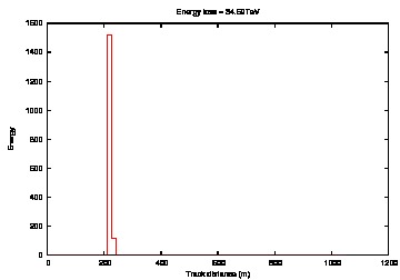
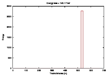
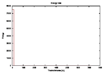
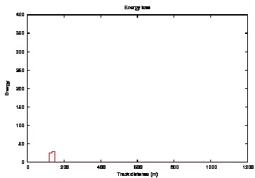
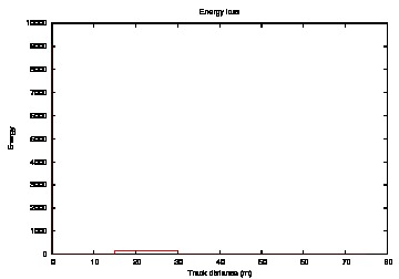
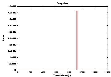
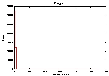
Can you use Nathan's energy estimator (millipede) on your final events to see if there is any evidence that there are muons sneaking through in these events?
Yes, I have done this thanks to Nathans help. Below you will see a "typical" muon event energy loss as well as both my remaining burn sample events. Both of these events have one clear, sharp peak with no evidence of a muon.
 |
 |
 |
 |
 |
 |
 |
 |
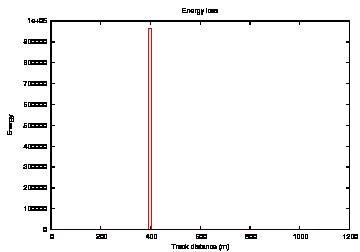 |
Figure 14: Millipede Energy estimator a) Run 110860, b) Run 111780, c) Typical muon, d) to i) Typical electron neutrino signal events.
Email from Jonathan, Thursday 21th April 2011, 10:18pm
I have been thinking a bit recently about the issues with DOMsimulator and DOMcalibrator. Including new software like WaveCalibrator is beyond what you should do, but what differences do you expect from these issues? Any qualitative ideas?
There were some bugs found (with DOMcalibrator saturation in particular) during the IC40 processing. Our processing was redone with corrections however, so these bugs are not present in this analysis. As for any effect that would happen had IC40 processing used modules that have been developed since then, I do not know what differences this would make.
What types of corsika survive to what points in your analysis? I tried to follow, and you have some plots on it in Level6. Some of this might be because I have a hard time telling colors in plots. I guess related is how many total MC events? Is including it in a table easy to do?
I have a table below that shows the number of events for each type of CORSIKA at level 4, 5 and 6.
| Type of CORSIKA | Level 4 | Level 5 | Level 6 |
| Single | 9,426 events | 694 events | 0 events |
| Double | 1,422 events | 120 events | 0 events |
| Triple | 97 events | 8 events | 0 events |
| Weighted Single | 380,545 events | 6,755 events | 0 events |
| Weighted Double | 1,472 events | 34 events | 0 events |
| Proton Two-component | n/a | 220 events | 0 events |
| Iron Two-component | n/a | 61 events | 0 events |
Table 1: Number of CORSIKA events at level 4, 5 and 6.
At level 4 you have a peak in your signal energy at 6.5, is this expected?
Yes, this is expected. It is the Glashow resonance which is unique to electron neutrinos and occurs at ~6.3 on logscale.
There seems to be a huge spike in data/corsika in the vertex plots (around -200,400) in your plot http://www2.phys.canterbury.ac.nz/~svh13/level5/IC40_L4_Cascade_2d_PosY_PosX_Plots.gif, why is this?
The peaks are due to the geometry of the strings. They occur where the detector is "pointy", particularly for the background. This is because in order for a muon to pass cut variable is has to look somewhat like a cascade and the easiest way for that to happen is for the muon track to just clip the edge of the detector so that the track is not seen. This happens a lot more easily at the "pointy" corners, and is the reason for my strong containment cuts.
You have a note about feature extractor bug, I wasn't here when it was discovered, how were the events from the EHE and muon streams chosen (to add to the cascade stream).
After the Feature Extractor bugs were found there was some concern that the cascade filter may have missed some events that should have been there. Events from the EHE and muon streams were re-evaluated to ensure that we caught any events that the cascade stream may have missed that should have been included.
In a few plots, there seems to be some data/mc mismatch. Like Credo_pos_z, do you know why?
Given the collaborations current ability to accurately simulate our background we can not avoid some data/MC discrepancy. It is more evident in some variables than others. In particular the reconstructed z vertex position due to the ice properties. Since I have no CORSIKA left after my final cut level, and I use the data for my limit on my background estimate this discrepancy does not affect the uncertainty in my results.
Doesn't your overtraining check show some overtraining (the background plots don't match well)?
Yes, there is some overtraining in the background. This is due to limited statistics which unfortunately I can do nothing about as I use all the standard CORSIKA that is available for IC40. The overtraining is not really much of a problem though since I do not reuse the CORSIKA that goes into the TMVA training for higher level analysis. I use the new two-component CORSIKA instead so I avoid any bias.
Does it help the BDT to have a clear variable cut which you don't make as an input, won't the BDT just make that quickly and clearly? Maybe put in all those events without that variable (despite it being so good) and see what other cuts the BDT uses to determine signal/background?
I'm not entirely sure what you mean here but the TMVA training uses all the variables without one being overly dominant. This is where the power of machine learning lies - it uses multi-dimentional parameter space and takes into account many variables in combination. If one variable is really dominant over all others the BDT result would not be as useful since one could just make that staight cut themselves without the additional variables information. Also if a variable is particularly strong a staight cut will not really make a difference since events that lie in the background region of that variable will get a very low BDT score so they are cut out anyway.
I look at your energy cuts (there is a 4.4 cut at the final level), does your low energy branch matter? How many signal/mc/data are getting through from it at the final levels? I am wondering how it effects the training of your BDT.
No, the low energy brach doesn't matter for my analysis. I also have a prelimiary cut on Energy before my TMVA training (in my level 4) at 3.4 on logscale so there are not many low energy events in the training of my BDT. The reason there is a low energy brach at all is because level 3 is a common level to the cascade working group. This means it is also used by all other cascade analyses, including low energy atmospheric searches such as Eike's and Doug's.
Thursday 21st April 2011, 10:30am
Henrike: Why do you not expand the region that you extrapolate from to get your CORSIKA background estimate? If you did this you may be able to use the CORSIKA for the extrapolation rather than the data.
I considered this. I can not expand the energy axis further as I have an energy cut at a previous level. The BDT axis can be expanded and I have tried this. However, there is still not sufficient CORSIKA to use for the extrapolation, and there is no benifit using data that is so far from the cut boundary for the extrapolation.
Patrick: Why are there peaks in the red line (level 5) in your livetime plot that are not present in the black line (level 4)?
This is to be expected. The livetime at level 5 is not a subset of the livetime at level 4 when binned by reconstructed energy. This is because livetime calculated by summing the weights: ∑ wi / ∑ wi2 and is therefore highly dependent on cut variables. On my Final webpage you will also see the livetime plots as a function of the MC Primary energy, where the liveimes are almost the same for each level because this is not a cut variable (and is only very loosely correlated with the reconstructed energy).
Gary: What is the actual number of the livetime for CORSIKA from your livetime plot?
From the two-component CORSIKA livetime plot (Figure 4d on my Final webpage) the total livetime at level 5 after an Energy cut at log10(CredoFit4_Energy) > 4.4 is 121.89 days. After the cuts BDT_MVA > 0.1 and log10(CredoFit4_Energy) > 3.4 the total livetime is 52.2452 days.
|